An Embedded Domain Specific Language for NXCALS and PM Queries

mmacieje · March 18, 2020, 5:52pm

Dear SWAN Users,

I am writing to share with you a package developed for simplifying query and processing of signals from Post Mortem, CALS, and NXCALS databases. The package was created as a part of the Signal Monitoring project I am involved in. The goal of this entry is to share the package with other users as some of you may find it useful in daily work.

The entry is an excerpt from API documentation also available as a SWAN notebook.

1. Logging Database Overview

Naturally, one should use a general purpose browser for ad-hoc queries and exploration for signal hierarchy:

The new PM web browser is available at the following link: http://post-mortem-paas.web.cern.ch/
The new TIMBER NXCALS web browser is available at: https://timber.cern.ch/
In order to find the mapping between CALS variables and NXCALS variable and metadata (along with the data migration status), please consult: https://ccde.cern.ch/dataBrowser/search?acwReportName=CALS-to-NXCALS%20Data%20Migration&domainName=CALS

In order to programatically query PM, CALS, or NXCALS database, a dedicated API along with parameters is required. An overview of databases from query perspective is summarised in the table below.

	PM	PM	CALS	CALS*	NXCALS	NXCALS
query type	event	signal	signal	feature	signal	feature
input	system, source, className	system, source, className, signal	signal	signal, features	system, (device, property), signal	system, (device, property), signal, features
time definition	time range	timestamp	time range	time range	time range	time range
time unit	ns	ns	s	s	ns	ns
return type	json	json	dict of list	dict of list	spark dataframe	spark dataframe
execution time	fast	fast	can be slow	fast	slow	fast
execution type	serial	serial	serial	?	serial	parallel
use	simple	simple	simple	simple	simple	requires good knowledge of pyspark

*The pytimber package provides an access to feature queries (for more details, please consult GitHub - rdemaria/pytimber: Python Wrapping of CALS API). Since CALS is about to be discontinued, we decided not to support this query in favor of NXCALS.

The native API for each database is available at:

PM REST API: http://pm-api-pro/
pytimber CALS API: GitHub - rdemaria/pytimber: Python Wrapping of CALS API
NXCALS python API: http://nxcals-docs.web.cern.ch/0.4.11/

2. Use of Native API to Query Signals in Python

Post Mortem REST API

import pandas as pd
import requests
import json

response = requests.get('http://pm-api-pro/v2/pmdata/signal?system=FGC&className=51_self_pmd&source=RPTE.UA47.RB.A45&timestampInNanos=1426220469520000000&signal=STATUS.I_MEAS')
json_response = json.loads(response.text)

name = json_response['content'][0]['namesAndValues'][0]['name']
time = json_response['content'][0]['namesAndValues'][1]['value']
value = json_response['content'][0]['namesAndValues'][0]['value']

pd.DataFrame(value, time, [name]).plot()

pm_native

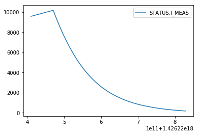
Note that for other systems the structure of returned json file may differ and requires dedicated handling

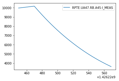
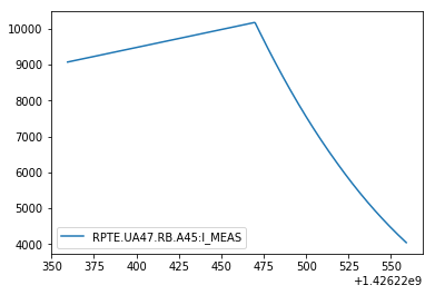
CALS pytimber API

import pandas as pd
import pytimber
ldb = pytimber.LoggingDB()

i_meas = ldb.get("RPTE.UA47.RB.A45:I_MEAS", '2015-03-13 05:20:49.4910002', '2015-03-13 05:22:49.4910002')
pd.DataFrame(i_meas.get("RPTE.UA47.RB.A45:I_MEAS")[1], i_meas.get("RPTE.UA47.RB.A45:I_MEAS")[0], ["RPTE.UA47.RB.A45:I_MEAS"]).plot()

cals_native

NXCALS API

from cern.nxcals.pyquery.builders import *
import pandas as pd

i_meas_df = DevicePropertyQuery.builder(spark).system('CMW') \
    .startTime(pd.Timestamp('2015-03-13T04:20:59.491000000').to_datetime64())\
    .endTime(pd.Timestamp('2015-03-13T04:22:49.491000000')) \
    .entity().device('RPTE.UA47.RB.A45').property('SUB') \
    .buildDataset().select('acqStamp', 'I_MEAS').dropna().sort("acqStamp").toPandas()

i_meas_df.set_index(i_meas_df['acqStamp'], inplace=True)
i_meas_df.drop(columns='acqStamp', inplace=True)
i_meas_df.plot()

nxcals_native

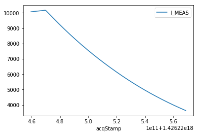
Note that signal query with NXCALS is quite time consuming.

3. pyeDSL - Embedded Domain Specific Language in Python

Use of the native API in larger analyses requires a lot of code and is difficult to generalise and introduce a structure for repeatable queries. Natural languages have certain structure [1].

Language	Word order	Example
English:	{Subject}.{Verb}.{Object}:	John ate cake
Japanese:	{Subject}.{Object}.{Verb}:	John-ga keiki-o tabeta
-	-	John cake ate

One can enforce syntactical order in code:

Domain Specific Language – new language, requires a parser
Embedded Domain Specific Language – extends existing language

Furthermore, an eDSL could be implemented following the Fluent interface approach [2]. The use of an eDSL for signal query and processing is not a new concept as there exists already an eDSL in Java used to automatically check signals during Hardware Commisionning campaigns of the LHC [3].

[1] K. Gulordava, Word order variation and dependency length minimisation: a cross-linguistic computational approach, PhD thesis, UniGe,
[2] Fluent interface - Wikipedia
[3] M. Audrain, et al. - Using a Java Embedded Domain-Specific Language for LHC Test Analysis, ICALEPCS2013, San Francisco, CA, USA

3.1. QueryBuilder

We propose a python embedded Domain Specific Language (pyeDSL) for building queries:

General purpose query

{DB}.{DURATION}.{QUERY_PARAMETERS}.{QUERY}

e.g.

df = QueryBuilder().{with_pm()/with_cals()/with_nxcals()}.with_duration().with_query_parameters()\
	.signal_query().dfs[0]
df = QueryBuilder().{with_pm()/with_cals()/with_nxcals()}.with_timestamp().with_query_parameters()\
	.signal_query().dfs[0]

Circuit-oriented query to generalize query across and within circuit types

{DB}.{DURATION}.{CIRCUIT_TYPE}.{METADATA}.{QUERY}

e.g.

df = QueryBuilder().{with_pm()/with_cals()/with_nxcals()}.with_duration().with_circuit_type().with_metadata()\
	.signal_query().dfs[0]
df = QueryBuilder().{with_pm()/with_cals()/with_nxcals()}.with_timestamp().with_circuit_type().with_metadata()\
	.signal_query().dfs[0]

With this approach:

each parameter defined once (validation of input at each stage)
single local variable is required
order of operation is fixed
vector inputs are supported

Furthermore, the pyeDSL provides hints on the order of execution

from lhcsmapi.pyedsl.QueryBuilder import QueryBuilder

QueryBuilder()

Set database name using with_pm(), with_cals(ldb), with_nxcals(spark) method.

from lhcsmapi.pyedsl.QueryBuilder import QueryBuilder

QueryBuilder().with_nxcals(spark)

Database name properly set to NXCALS. Set time definition: for PM signal query, with_timestamp(),
for PM event query or CALS, NXCALS signal query, with_duration()

from lhcsmapi.pyedsl.QueryBuilder import QueryBuilder

QueryBuilder().with_nxcals(spark).with_duration(t_start='2015-03-13 05:20:59.4910002', duration=[(100, 's'), (100, 's')])

Query duration set to t_start=1426220359491000200, t_end=1426220559491000200. Set generic query parameter using with_query_parameters() method, or a circuit signal using with_circuit_type() method.

At the same time it prohibits unsupported operations throwing a meaningful exception.

from lhcsmapi.pyedsl.QueryBuilder import QueryBuilder

QueryBuilder().with_duration(t_start='2015-03-13 05:20:59.4910002', duration=[(100, 's'), (100, 's')])

AttributeError: with_duration() is not supported. Set database name using with_pm(), with_cals(ldb), with_nxcals(spark) method.

A sentence constructed this way maintains the differences of query types while providing a common structure.

3.1.1. PM Event Query

Allows finding source and timestamp of PM events within a period of time.

from lhcsmapi.pyedsl.QueryBuilder import QueryBuilder

source_timestamp_df = QueryBuilder().with_pm() \
    .with_duration(t_start='2015-03-13 05:20:59.4910002', duration=[(100, 's'), (100, 's')]) \
    .with_query_parameters(system='FGC', className='51_self_pmd', source='RPTE.UA47.RB.A45') \
    .event_query().df

source_timestamp_df

	source	timestamp
0	RPTE.UA47.RB.A45	1426220469520000000

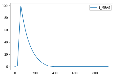
3.1.2. PM Signal Query

Queries signal based on a timestamp as well as system, source, className, and signal.

from lhcsmapi.pyedsl.QueryBuilder import QueryBuilder

i_meas_df = QueryBuilder().with_pm() \
    .with_timestamp(1426220469520000000) \
    .with_query_parameters(system='FGC', source='RPTE.UA47.RB.A45', className='51_self_pmd', signal='STATUS.I_MEAS') \
    .signal_query().dfs[0]

i_meas_df.plot()

pm_native

3.1.3. CALS Signal Query

Queries signal based on a time duration as well as signal.

from lhcsmapi.pyedsl.QueryBuilder import QueryBuilder
import pytimber
ldb = pytimber.LoggingDB()

i_meas_df = QueryBuilder().with_cals(ldb) \
    .with_duration(t_start='2015-03-13 05:20:59.4910002', duration=[(100, 's'), (100, 's')]) \
    .with_query_parameters(signal='RPTE.UA47.RB.A45:I_MEAS') \
    .signal_query().dfs[0]

i_meas_df.plot()

cals_pyedsl

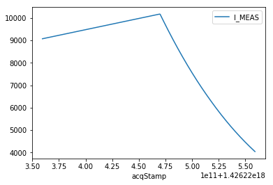
3.1.4. NXCALS Signal Query

Queries signal based on a time duration as well as system, device, property, and signal.

from lhcsmapi.pyedsl.QueryBuilder import QueryBuilder

i_meas_df = QueryBuilder().with_nxcals(spark) \
    .with_duration(t_start='2015-03-13 05:20:59.4910002', duration=[(100, 's'), (100, 's')]) \
    .with_query_parameters(nxcals_system='CMW', nxcals_device='RPTE.UA47.RB.A45', nxcals_property='SUB', signal='I_MEAS') \
    .signal_query().dfs[0]

i_meas_df.plot()

nxcals_pyedsl_device_property

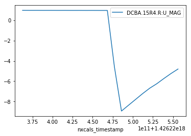
Queries signal based on a time duration as well as system and signal.

from lhcsmapi.pyedsl.QueryBuilder import QueryBuilder

u_mag_df = QueryBuilder().with_nxcals(spark) \
    .with_duration(t_start='2015-03-13 05:20:59.4910002', duration=[(100, 's'), (100, 's')]) \
    .with_query_parameters(nxcals_system='WINCCOA', signal='DCBA.15R4.R:U_MAG') \
    .signal_query().dfs[0]

u_mag_df.plot()

nxcals_pyedsl_variable

3.1.5. NXCALS Feature Query

Queries signal features (mean, std, max, min, count) based on a time duration as well as system, device, property, and signal.

from lhcsmapi.pyedsl.QueryBuilder import QueryBuilder

i_meas_df = QueryBuilder().with_nxcals(spark) \
    .with_duration(t_start=1526898157236000000, t_end=1526903352338000000) \
    .with_query_parameters(nxcals_system='CMW', nxcals_device='RPTE.UA23.RB.A12', nxcals_property='SUB', signal='I_MEAS') \
    .feature_query(['mean', 'std', 'max', 'min', 'count']).df

i_meas_df

	device	max	min	count	mean	std
0	RPTE.UA23.RB.A12	10978.8	757.18	2498	5374.768659	3315.972856

The same query with native NXCALS API is

i_meas_results_ds = DevicePropertyQuery.builder(spark).system('CMW') \
    .startTime(t_start_injs).endTime(t_end_sbs) \
    .entity().device('RPTE.UA23.RB.A12').property('SUB') \
    .buildDataset().select("acqStamp", 'I_MEAS', "device") \
    .agg(func.mean('I_MEAS'), func.stddev('I_MEAS'), func.max('I_MEAS'), 
         func.min('I_MEAS'), func.count('I_MEAS')).collect()

i_meas_results_df = pd.DataFrame(i_meas_results_ds, columns=['I_MEAS_device', 'I_MEAS_class', 'I_MEAS_mean', 'I_MEAS_std', 'I_MEAS_max', 'I_MEAS_min', 'I_MEAS_count']).sort_values(by=['I_MEAS_class'])
i_meas_results_df

Queries signal features (mean, std, max, min, count) based on a time duration as well as system and signal.

from lhcsmapi.pyedsl.QueryBuilder import QueryBuilder

u_mag_df = QueryBuilder().with_nxcals(spark) \
    .with_duration(t_start=1526898157236000000, t_end=1526903352338000000) \
    .with_query_parameters(nxcals_system='WINCCOA', signal='DCBB.8L2.R:U_MAG') \
    .feature_query(['mean', 'std', 'max', 'min', 'count']).df

u_mag_df

	nxcals_variable_name	max	min	count	mean	std
0	DCBB.8L2.R:U_MAG	0.002113	-0.975332	51951	-0.196706	0.375195

3.2. Polymorphism

pyeDSL allows for processing of lists of signal definitions.

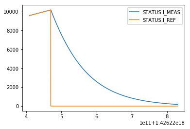
multiple signal, mutliple sources, multiple systems, multiple className

from lhcsmapi.pyedsl.QueryBuilder import QueryBuilder

i_meas_df = QueryBuilder().with_pm() \
    .with_timestamp(1426220469520000000) \
    .with_query_parameters(system=['FGC', 'FGC'], source=['RPTE.UA47.RB.A45', 'RPTE.UA47.RB.A45'], 
                           className=['51_self_pmd', '51_self_pmd'], signal=['STATUS.I_MEAS', 'STATUS.I_REF']) \
    .signal_query().dfs

ax=i_meas_df[0].plot()
i_meas_df[1].plot(ax=ax)

pm_pyedsl_polymorphism_1

multiple signal, single source, single system, single className

from lhcsmapi.pyedsl.QueryBuilder import QueryBuilder

i_meas_df = QueryBuilder().with_pm() \
    .with_timestamp(1426220469520000000) \
    .with_query_parameters(system='FGC', source='RPTE.UA47.RB.A45', 
                           className='51_self_pmd', signal=['STATUS.I_MEAS', 'STATUS.I_REF']) \
    .signal_query().dfs

ax=i_meas_df[0].plot()
i_meas_df[1].plot(ax=ax)

pm_pyedsl_polymorphism_1

3.3. Advanced Feature Query

NXCALS enables calculation of signal features such as min, max, mean, std, count directly on the cluster without the need for costly query of the signal and performing calculation locally. This approach enables parallel computing on the cluster. To this end, a query should contain an element enabling a group by operation. Each group by operation allows for executing computation in parallel.

Feature query of multiple signals for the same period of time

from lhcsmapi.pyedsl.QueryBuilder import QueryBuilder

i_meas_df = QueryBuilder().with_nxcals(spark) \
    .with_duration(t_start=1526898157236000000, t_end=1526903352338000000) \
    .with_circuit_type('RB') \
    .with_metadata(circuit_name='*', system='PC', signal='I_MEAS') \
    .feature_query(['mean', 'std', 'max', 'min', 'count']).df

i_meas_df

	device	max	min	count	mean	std
0	RPTE.UA63.RB.A56	10974.36	756.90	2498	5372.636369	3314.646638
1	RPTE.UA87.RB.A81	10973.21	756.82	2498	5371.596990	3314.230379
2	RPTE.UA83.RB.A78	10967.94	756.47	2498	5369.226934	3312.676833
3	RPTE.UA27.RB.A23	10976.46	757.04	2498	5373.973151	3315.324716
4	RPTE.UA43.RB.A34	10975.16	756.95	2497	5373.559131	3314.074552
5	RPTE.UA67.RB.A67	10978.56	757.18	2498	5374.329179	3315.855302
6	RPTE.UA47.RB.A45	10971.44	756.71	2497	5370.954557	3312.837184
7	RPTE.UA23.RB.A12	10978.80	757.18	2498	5374.768659	3315.972856

Feature query of multiple signals with the same period of time subdivided into three intervals - group by signal name and interval

t_start_injs = 1526898157236000000
t_end_injs = 1526899957236000000
t_start_sbs = 1526901552338000000
t_end_sbs = 1526903352338000000

from lhcsmapi.pyedsl.QueryBuilder import QueryBuilder

i_meas_df = QueryBuilder().with_nxcals(spark) \
    .with_duration(t_start=t_start_injs, t_end=t_end_sbs) \
    .with_circuit_type('RB') \
    .with_metadata(circuit_name='RB.A12', system='PC', signal='I_MEAS')\
    .signal_query().dfs[0]

ax = i_meas_df.plot(figsize=(10,5), linewidth=5)
ax.axvspan(xmin=t_start_injs, xmax=t_end_injs, facecolor='xkcd:goldenrod')
ax.axvspan(xmin=t_end_injs, xmax=t_start_sbs, facecolor='xkcd:grey')
ax.axvspan(xmin=t_start_sbs, xmax=t_end_sbs, facecolor='xkcd:green')

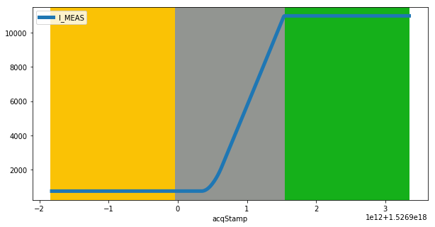
nxcals_pyedsl_feature_query_translate

Function translate introduces a mapping based on the time column. Here, we consider three subintervals for beam injection, beam acceleration, and stable beams.

As a result, the time column forms a partition and can be executed in parallel.

from pyspark.sql.functions import udf
from pyspark.sql.types import IntegerType

def translate(timestamp):
    if(timestamp >= t_start_injs and timestamp < t_end_injs):
        return 1
    
    if(timestamp >=  t_end_injs and timestamp < t_start_sbs):
        return 2
    
    if(timestamp >= t_start_sbs and timestamp <= t_end_sbs):
        return 3
    
    return -1

translate_udf = udf(translate, IntegerType())

The translate function should be passed as a function argument

i_meas_df = QueryBuilder().with_nxcals(spark) \
    .with_duration(t_start=t_start_injs, t_end=t_end_sbs) \
    .with_circuit_type('RB') \
    .with_metadata(circuit_name='*', system='PC', signal='I_MEAS') \
    .feature_query(['mean', 'std', 'max', 'min', 'count'], function=translate_udf).df

i_meas_df.head()

	device	class	max	min	count	mean	std
0	RPTE.UA43.RB.A34	1	756.96	756.95	60	756.959833	0.001291
1	RPTE.UA63.RB.A56	3	10974.36	10974.35	60	10974.350167	0.001291
2	RPTE.UA47.RB.A45	3	10971.44	10971.43	60	10971.439667	0.001810
3	RPTE.UA47.RB.A45	2	10970.89	756.71	2377	5346.059971	3193.562789

The same method applied to NXCALS signals based on variable

from lhcsmapi.pyedsl.QueryBuilder import QueryBuilder

u_mag_ab_df = QueryBuilder().with_nxcals(spark) \
    .with_duration(t_start=t_start_injs, t_end=t_end_sbs) \
    .with_circuit_type('RB') \
    .with_metadata(circuit_name='RB.A12', system='BUSBAR', signal='U_MAG', wildcard={'BUSBAR': 'DCBB.8L2.R'}) \
    .feature_query(['mean', 'std', 'max', 'min', 'count'], function=translate_udf).df

u_mag_ab_df

	nxcals_variable_name	class	max	min	count	mean	std
0	DCBB.8L2.R:U_MAG	3	0.002003	-0.034035	18000	-0.001983	0.002882
1	DCBB.8L2.R:U_MAG	1	0.002113	-0.005992	18000	-0.001861	0.002844
2	DCBB.8L2.R:U_MAG	2	0.002041	-0.975332	15951	-0.636315	0.423767

This method can be used together with signal decimation, i.e., taking every nth sample.

For example this can be useful to query QPS board A and B which share the same channel and samples are shifted by 5 so that

every 10-th sample belongs to board A (or B), decimation=10

from lhcsmapi.pyedsl.QueryBuilder import QueryBuilder

u_mag_a_df = QueryBuilder().with_nxcals(spark) \
    .with_duration(t_start=t_start_injs, t_end=t_end_sbs) \
    .with_circuit_type('RB') \
    .with_metadata(circuit_name='RB.A12', system='BUSBAR', signal='U_MAG', wildcard={'BUSBAR': 'DCBB.8L2.R'}) \
    .feature_query(['mean', 'std', 'max', 'min', 'count'], function=translate_udf, decimation=10).df

u_mag_a_df

	nxcals_variable_name	class	max	min	count	mean	std
0	DCBB.8L2.R:U_MAG	3	0.002003	-0.012705	1800	0.000812	0.000529
1	DCBB.8L2.R:U_MAG	1	0.002113	-0.000463	1800	0.000965	0.000434
2	DCBB.8L2.R:U_MAG	2	0.002041	-0.969405	1595	-0.633601	0.423847

every 5+10-th sample belongs to board B (or A), decimation=10, shift=5

from lhcsmapi.pyedsl.QueryBuilder import QueryBuilder

u_mag_b_df = QueryBuilder().with_nxcals(spark) \
    .with_duration(t_start=t_start_injs, t_end=t_end_sbs) \
    .with_circuit_type('RB') \
    .with_metadata(circuit_name='RB.A12', system='BUSBAR', signal='U_MAG', wildcard={'BUSBAR': 'DCBB.8L2.R'}) \
    .feature_query(['mean', 'std', 'max', 'min', 'count'], function=translate_udf, decimation=10, shift=5).df

u_mag_b_df

	nxcals_variable_name	class	max	min	count	mean	std
0	DCBB.8L2.R:U_MAG	3	-0.003425	-0.034035	1800	-0.004754	0.000877
1	DCBB.8L2.R:U_MAG	1	-0.003361	-0.005992	1800	-0.004656	0.000441
2	DCBB.8L2.R:U_MAG	2	-0.003052	-0.975332	1595	-0.639233	0.423941

with polymorphism one can query 1248 busbar at once (in two batches of 624 due to the limit of 1000 signal per query)

from lhcsmapi.pyedsl.QueryBuilder import QueryBuilder

u_mag_ab_df = QueryBuilder().with_nxcals(spark) \
    .with_duration(t_start=t_start_injs, t_end=t_end_sbs) \
    .with_circuit_type('RB') \
    .with_metadata(circuit_name='*', system='BUSBAR', signal='U_MAG', wildcard={'BUSBAR': '*'}) \
    .feature_query(['mean', 'std', 'max', 'min', 'count'], function=translate_udf).df

u_mag_ab_df.head()

	nxcals_variable_name	class	max	min	count	mean	std
0	DCBA.22L4.L:U_MAG	1	-0.000167	-0.002102	18000	-0.001110	0.000639
1	DCBA.14L4.R:U_MAG	1	0.001179	-0.000796	18000	0.000171	0.000603
2	DCBA.A28R2.L:U_MAG	3	0.045531	-0.003455	18000	-0.002131	0.001361
3	DCBB.B22L2.R:U_MAG	1	0.000341	-0.003088	18000	-0.001283	0.000557
4	DCBB.11L2.R:U_MAG	3	0.048651	-0.002121	18000	0.001457	0.002587

3.4. Processing Raw Signals

Once a signal is queried, one can perform some operations on each of them.
In this case, the order of operations does not matter (but can be checked).

Signal query	Signal processing
{DB}.{DURATION}.{QUERY_PARAMETERS}.{QUERY}
{DB}.{DURATION}.{CIRCUIT_TYPE}.{METADATA}.{QUERY}
	.synchronize_time()
	.convert_index_to_sec()
	.create_col_from_index()
	.filter_median()
	.remove_values_for_time_less_than()
	.remove_initial_offset()

from lhcsmapi.pyedsl.QueryBuilder import QueryBuilder

i_meas_df = QueryBuilder().with_nxcals(spark) \
    .with_duration(t_start='2015-01-13 16:59:11+01:00', t_end='2015-01-13 17:15:46+01:00') \
    .with_circuit_type('RB') \
    .with_metadata(circuit_name='RB.A12', system='PC', signal='I_MEAS') \
    .signal_query() \
    .synchronize_time() \
    .convert_index_to_sec().dfs[0]

i_meas_df.plot()

pm_pyedsl_signal_processing

etejedor · March 18, 2020, 6:11pm

Hi,

This is wonderful, would you like to add the notebook (and potentially other notebooks as well) to a SWAN gallery directly accessible from SWAN (via the galleries icon on the top bar)?

This way the interested users would be able to find in SWAN the explanation on how to use the package.

mmacieje · March 18, 2020, 6:13pm

Hi Enric,

absolutely, I’ll add the notebook to the gallery tomorrow. Thank you for a positive response.

Cheers, Michał.